Pauli matrices

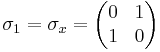
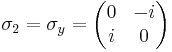
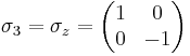
The Pauli matrices are a set of three 2 × 2 complex matrices which are Hermitian and unitary.^[1] Usually indicated by the Greek letter "sigma" (σ), they are occasionally denoted with a "tau" (τ) when used in connection with isospin symmetries. They are:

$\sigma_1 = \sigma_x = \begin{pmatrix} 0&1\\ 1&0 \end{pmatrix}$

$\sigma_2 = \sigma_y = \begin{pmatrix} 0&-i\\ i&0 \end{pmatrix}$

$\sigma_3 = \sigma_z = \begin{pmatrix} 1&0\\ 0&-1 \end{pmatrix}$

These matrices were used by, then named after, the Austrian-born physicist Wolfgang Pauli (1900–1958), in his study of spin in quantum mechanics.

Each Pauli matrix is Hermitian, and together with the identity I (sometimes considered the zeroth Pauli matrix $\sigma_0$ ), the Pauli matrices span the full vector space of 2x2 Hermitian matrices. In the language of quantum mechanics, hermitian matrices are observables, so the Pauli matrices span the space of observables of the 2-dimensional complex Hilbert space. In the context of Pauli's work, $\sigma_i$ is the observable corresponding to spin along the $i^{th}$ coordinate axis in $\mathbb{R}^3$ .

The Pauli matrices (after multiplication by i to make them anti-hermitian), also generate transformations in the sense of Lie algebras: the matrices $i\sigma_1,i\sigma_2,i\sigma_3$ form a basis for $\mathfrak{su}_2$ , which exponentiates to the spin group $SU(2)$ , and for the identical Lie algebra $\mathfrak{so_3}$ , which exponentiates to the Lie group $SO(3)$ of rotations of 3-dimensional space. Moreover, the algebra generated by the four matrices 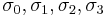$\sigma_0,\sigma_1,\sigma_2,\sigma_3$ forms a faithful representation of the 3-dimensional real, Euclidean Clifford Algebra.

1 Algebraic properties
2 SU(2)
3 Physics
- 3.1 Quantum mechanics
- 3.2 Quantum information
4 See also
5 Notes
6 References

Algebraic properties

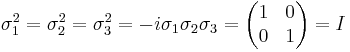
$\sigma_1^2 = \sigma_2^2 = \sigma_3^2 = -i\sigma_1 \sigma_2 \sigma_3 = \begin{pmatrix} 1&0\\0&1\end{pmatrix} = I$

where I is the identity matrix, i.e. the matrices are involutory.

The determinants and traces of the Pauli matrices are:

$\det (\sigma_i) = -1,$

$\operatorname{Tr} (\sigma_i) = 0 .$

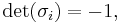
From above we can deduce that the eigenvalues of each σ_i are ±1.

Together with the identity matrix I (which is sometimes written as σ₀), the Pauli matrices form an orthogonal basis, in the sense of Hilbert-Schmidt, for the real Hilbert space of 2 × 2 complex Hermitian matrices, or the complex Hilbert space of all 2 × 2 matrices.

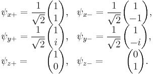
Eigenvectors and eigenvalues

Each of the (hermitian) Pauli matrices has two eigenvalues, +1 and −1. The corresponding normalized eigenvectors are:

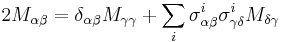
$\begin{array}{lclc} \psi_{x%2B}=\displaystyle\frac{1}{\sqrt{2}}\!\!\!\!\! & \begin{pmatrix}{1}\\{1}\end{pmatrix}, & \psi_{x-}=\displaystyle\frac{1}{\sqrt{2}}\!\!\!\!\! & \begin{pmatrix}{1}\\{-1}\end{pmatrix}, \\ \psi_{y%2B}=\displaystyle\frac{1}{\sqrt{2}}\!\!\!\!\! & \begin{pmatrix}{1}\\{i}\end{pmatrix}, & \psi_{y-}=\displaystyle\frac{1}{\sqrt{2}}\!\!\!\!\! & \begin{pmatrix}{1}\\{-i}\end{pmatrix}, \\ \psi_{z%2B}= & \begin{pmatrix}{1}\\{0}\end{pmatrix}, & \psi_{z-}= & \begin{pmatrix}{0}\\{1}\end{pmatrix}. \end{array}$

Pauli vector

The Pauli vector is defined by

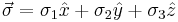
$\vec{\sigma} = \sigma_1 \hat{x} %2B \sigma_2 \hat{y} %2B \sigma_3 \hat{z} \,$

and provides a mapping mechanism from a vector basis to a Pauli matrix basis as follows

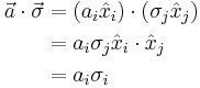
$\begin{align} \vec{a} \cdot \vec{\sigma} &= (a_i \hat{x}_i) \cdot (\sigma_j \hat{x}_j ) \\ &= a_i \sigma_j \hat{x}_i \cdot \hat{x}_j \\ &= a_i \sigma_i \end{align}$

(summation over indices implied). Note that in this vector dotted with Pauli vector operation the Pauli matrices are treated in a scalar like fashion, commuting with the vector basis elements.

Commutation relations

The Pauli matrices obey the following commutation and anticommutation relations:

$[\sigma_a, \sigma_b] = 2 i \varepsilon_{a b c}\,\sigma_c,$

$\{\sigma_a, \sigma_b\} = 2 \delta_{a b} \cdot I.$

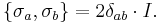
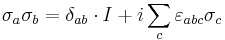
where $\varepsilon_{abc}$ is the Levi-Civita symbol, $\delta_{ab}$ is the Kronecker delta, and I is the identity matrix.

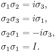
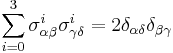
The above two relations are equivalent to:

$\sigma_a \sigma_b = \delta_{ab} \cdot I %2B i \sum_c \varepsilon_{abc} \sigma_c \,$ .

For example,

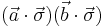
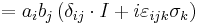
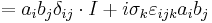
$\begin{align} \sigma_1\sigma_2 &= i\sigma_3,\\ \sigma_2\sigma_3 &= i\sigma_1,\\ \sigma_2\sigma_1 &= -i\sigma_3,\\ \sigma_1\sigma_1 &= I.\\ \end{align}$

and the summary equation for the commutation relations can be used to prove

$(\vec{a} \cdot \vec{\sigma})(\vec{b} \cdot \vec{\sigma}) = (\vec{a} \cdot \vec{b}) \, I %2B i \vec{\sigma} \cdot ( \vec{a} \times \vec{b} ) \quad \quad \quad \quad (1) \,$

(as long as the vectors a and b commute with the pauli matrices)

as well as

$e^{i (\vec{a} \cdot \vec{\sigma})} = I\cos{a} %2B i (\hat{n} \cdot \vec{\sigma}) \sin{a} \quad \quad \quad \quad \quad \quad (2) \,$

for $\vec{a} = a \hat{n}$ .

Proof of (1)

$(\vec{a} \cdot \vec{\sigma})(\vec{b} \cdot \vec{\sigma}) \,$	$= a_i \sigma_i b_j \sigma_j \,$
	$= a_i b_j \sigma_i \sigma_j \,$
	$= a_i b_j \left( \delta_{ij} \cdot I%2B i \varepsilon_{ijk} \sigma_k \right) \,$
	$= a_i b_j \delta_{ij} \cdot I%2B i \sigma_k \varepsilon_{ijk} a_i b_j \,$
	$= ( \vec{a} \cdot \vec{b} ) \cdot I%2B i \vec{\sigma} \cdot ( \vec{a} \times \vec{b} )\,$

Proof of (2)

First notice that for even powers

$(\hat{n} \cdot \vec{\sigma})^{2n} = I \,$

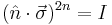
but for odd powers

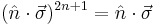
$(\hat{n} \cdot \vec{\sigma})^{2n%2B1} = \hat{n} \cdot \vec{\sigma} \,$

Combine these two facts with the knowledge of the relation of the exponential to sine and cosine:

$e^{ix} \,$	$= \sum_{n=0}^\infty{\frac{i^n x^n}{n!}} \,$
	$= \sum_{n=0}^\infty{\frac{(-1)^n x^{2n}}{(2n)!}} %2B i\sum_{n=0}^\infty{\frac{(-1)^n x^{2n%2B1}}{(2n%2B1)!}} \,$

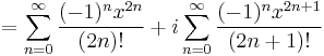
Which, when we use 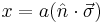$x = a (\hat{n} \cdot \vec{\sigma}) \,$ gives us

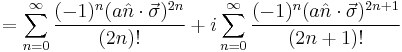
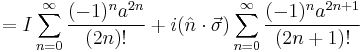
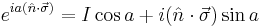
$= \sum_{n=0}^\infty{\frac{(-1)^n (a\hat{n}\cdot \vec{\sigma})^{2n}}{(2n)!}} %2B i\sum_{n=0}^\infty{\frac{(-1)^n (a\hat{n}\cdot \vec{\sigma})^{2n%2B1}}{(2n%2B1)!}} \,$

$= I\sum_{n=0}^\infty{\frac{(-1)^n a^{2n}}{(2n)!}} %2B i (\hat{n}\cdot \vec{\sigma}) \sum_{n=0}^\infty{\frac{(-1)^n a^{2n%2B1}}{(2n%2B1)!}} \,$

The sum on the left is cosine, and the sum on the right is sine so finally,

$e^{i a(\hat{n} \cdot \vec{\sigma})} = I\cos{a} %2B i (\hat{n} \cdot \vec{\sigma}) \sin{a} \,$

Completeness relation

An alternative notation that is commonly used for the Pauli matrices is to write the vector index $i$ in the superscript, and the matrix indices as subscripts, so that the element in row $\alpha$ and column $\beta$ of the $i$ ^th Pauli matrix is $\sigma^i_{\alpha\beta}$ .

In this notation, the completeness relation for the Pauli matrices can be written

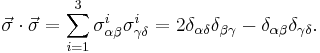
$\vec{\sigma}\cdot\vec{\sigma}=\sum_{i=1}^3 \sigma^i_{\alpha\beta}\sigma^i_{\gamma\delta} = 2 \delta_{\alpha\delta} \delta_{\beta\gamma} - \delta_{\alpha\beta}\delta_{\gamma\delta}.\,$

Proof

The fact that the Pauli matrices, along with the identity matrix $I$ , form an orthogonal basis for the complex Hilbert space of all 2 × 2 matrices mean that we can express any matrix $M$ as

$M = c \mathbf{I} %2B \sum_i a_i \sigma^i$

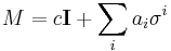
where $c$ is a complex number, and $a$ is a 3-component complex vector. It is straightforward to show, using the properties listed above, that

$\mathrm{tr}\, \sigma^i\sigma^j = 2\delta_{ij}$

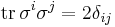
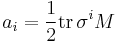where $\mathrm{tr}$ denotes the trace, and hence that $c=\frac{1}{2}\mathrm{tr}\,M$ and $a_i = \frac{1}{2}\mathrm{tr}\,\sigma^i M$ . This therefore gives

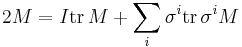
$2M = I \mathrm{tr}\, M %2B \sum_i \sigma^i \mathrm{tr}\, \sigma^i M$

which can be rewritten in terms of matrix indices as

$2M_{\alpha\beta} = \delta_{\alpha\beta} M_{\gamma\gamma} %2B \sum_i \sigma^i_{\alpha\beta} \sigma^i_{\gamma\delta} M_{\delta\gamma}$

where summation is implied over the repeated indices $\gamma$ and $\delta$ . Since this is true for any choice of the matrix $M$ , the completeness relation follows as stated above.

As noted above, it is common to denote the $2\times2$ unit matrix by $\sigma_0$ , so $\sigma^0_{\alpha\beta} = \delta_{\alpha\beta}$ . The completeness relation can therefore alternatively be expressed as

$\sum_{i=0}^3 \sigma^i_{\alpha\beta}\sigma^i_{\gamma\delta} = 2 \delta_{\alpha\delta} \delta_{\beta\gamma}\,$ .

Relation with the permutation operator

Let $P_{ij}$ be the permutation (transposition, actually) between two spins $\sigma_i$ and $\sigma_j$ living in the tensor product space 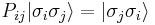$\mathbb{C}^2 \otimes \mathbb{C}^2$ , $P_{ij}|\sigma_i \sigma_j\rangle = |\sigma_j \sigma_i\rangle$ . This operator can be written as 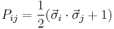$P_{ij} = \frac{1}{2}(\vec{\sigma}_i\cdot\vec{\sigma}_j%2B1)$ , as the reader can easily verify.

SU(2)

The matrix group SU(2) is a Lie group, and its Lie algebra is the set of the anti-Hermitian 2×2 matrices with trace 0. Direct calculation shows that the Lie algebra su(2) is the 3 dimensional real algebra spanned by the set { $i \sigma_j$ }. In symbols,

$\; \operatorname{su}(2) = \operatorname{span} \{ i \sigma_1, i \sigma_2 , i \sigma_3 \}.$

As a result, $i \sigma_j$ s can be seen as infinitesimal generators of SU(2).

A Cartan decomposition of SU(2)

This relationship between the Pauli matrices and SU(2) can be explored further, as can be seen from the following simple example. We can write

$\; \operatorname{su}(2) = \operatorname{span} \{i \sigma_2\} \oplus \operatorname{span} \{ i \sigma_1, i \sigma_3\}.$

We put

$\; \mathfrak{k} = \operatorname{span} \{i \sigma_3\},$

and

$\; \mathfrak{p} = \operatorname{span} \{ i \sigma_1, i \sigma_2\}.$

Using the algebraic identities listed in the previous section, it can be verified that $\mathfrak{k}$ and $\mathfrak{p}$ form a Cartan pair of the Lie algebra SU(2). Furthermore,

$\; \mathfrak{a} = \operatorname{span} \{ i \sigma_2\}$

is a maximal abelian subalgebra of $\mathfrak{p}$ . Now, a version of Cartan decomposition states that any element U in the Lie group SU(2) can be expressed in the form

$U = e^{k_1} e^a e^{k_2}\,\!$ where $k_1, k_2 \in \mathfrak{k}$ and $a \in \mathfrak{a}.$

In other words, any unitary U of determinant 1 is of the form

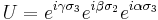
$U = e^{i \gamma \sigma_3} e^{i \beta \sigma_2} e^{i \alpha \sigma_3}\,\!$

for some real numbers α, β, and γ. Physically, this corresponds to the important z-y-z decomposition of a general 3D rotation.

Extending to unitary matrices gives that any unitary 2 × 2 U is of the form

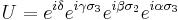
$U = e^{i \delta} e^{i \gamma \sigma_3} e^{i \beta \sigma_2} e^{i \alpha \sigma_3}\,\!$

where the additional parameter δ is also real (also compare with Leonhardt 2010, eq 5.22, pg. 99)

SO(3)

The Lie algebra su(2) is isomorphic to the Lie algebra so(3), which corresponds to the Lie group SO(3), the group of rotations in three-dimensional space. In other words, one can say that $i \sigma_j$ 's are a realization (and, in fact, the lowest-dimensional realization) of infinitesimal rotations in three-dimensional space. However, even though su(2) and so(3) are isomorphic as Lie algebras, SU(2) and SO(3) are not isomorphic as Lie groups. SU(2) is actually a double cover of SO(3), meaning that there is a two-to-one homomorphism from SU(2) to SO(3).

Quaternions

The real linear span of 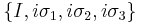$\{I, i\sigma_1, i\sigma_2, i\sigma_3\}\,$ is isomorphic to the real algebra of quaternions H. The isomorphism from H to this set is given by the following map (notice the reversed signs for the Pauli matrices):

$1 \mapsto I, \quad i \mapsto - i \sigma_1, \quad j \mapsto - i \sigma_2, \quad k \mapsto - i \sigma_3.$

Alternatively, the isomorphism can be achieved by a map using the Pauli matrices in reversed order,^[2]

$1 \mapsto I, \quad i \mapsto i \sigma_3, \quad j \mapsto i \sigma_2, \quad k \mapsto i \sigma_1.$

As the quaternions of unit norm is group-isomorphic to SU(2), this gives yet another way of describing SU(2) via the Pauli matrices. The two-to-one homomorphism from SU(2) to SO(3) can also be explicitly given in terms of the Pauli matrices in this formulation.

Quaternions form a division algebra—every non-zero element has an inverse—whereas Pauli matrices do not. For a quaternionic version of the algebra generated by Pauli matrices see biquaternions, which is a venerable algebra of eight real dimensions.

Physics

Quantum mechanics

In quantum mechanics, each Pauli matrix is related to an operator that corresponds to an observable describing the spin of a spin ½ particle, in each of the three spatial directions. Also, as an immediate consequence of the Cartan decomposition mentioned above, $i \sigma_j$ are the generators of rotation acting on non-relativistic particles with spin ½. The state of the particles are represented as two-component spinors. An interesting property of spin ½ particles is that they must be rotated by an angle of 4 $\pi$ in order to return to their original configuration. This is due to the two-to-one correspondence between SU(2) and SO(3) mentioned above, and the fact that, although one visualizes spin up/down as the north/south pole on the 2-sphere S², they are actually represented by orthogonal vectors in the two dimensional complex Hilbert space.

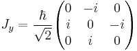
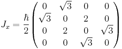
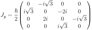
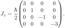
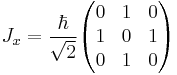
For a spin ½ particle, the spin operator is given by $\mathbf{J} =\frac\hbar2\boldsymbol{\sigma}$ . It is possible to form generalizations of the Pauli matrices in order to describe higher spin systems in three spatial dimensions. The spin matrices for spin 1 and spin $\frac{3}{2}$ are given below:

$j=1$ :

$J_x = \frac{\hbar}{\sqrt{2}} \begin{pmatrix} 0&1&0\\ 1&0&1\\ 0&1&0 \end{pmatrix}$

$J_y = \frac{\hbar}{\sqrt{2}} \begin{pmatrix} 0&-i&0\\ i&0&-i\\ 0&i&0 \end{pmatrix}$

$J_z = \hbar \begin{pmatrix} 1&0&0\\ 0&0&0\\ 0&0&-1 \end{pmatrix}$

$j=\textstyle\frac{3}{2}$ :

$J_x = \frac\hbar2 \begin{pmatrix} 0&\sqrt{3}&0&0\\ \sqrt{3}&0&2&0\\ 0&2&0&\sqrt{3}\\ 0&0&\sqrt{3}&0 \end{pmatrix}$

$J_y = \frac\hbar2 \begin{pmatrix} 0&-i\sqrt{3}&0&0\\ i\sqrt{3}&0&-2i&0\\ 0&2i&0&-i\sqrt{3}\\ 0&0&i\sqrt{3}&0 \end{pmatrix}$

$J_z = \frac\hbar2 \begin{pmatrix} 3&0&0&0\\ 0&1&0&0\\ 0&0&-1&0\\ 0&0&0&-3 \end{pmatrix}.$

Also useful in the quantum mechanics of multiparticle systems, the general Pauli group G_n is defined to consist of all n-fold tensor products of Pauli matrices.

The fact that any 2 × 2 complex Hermitian matrices can be expressed in terms of the identity matrix and the Pauli matrices also leads to the Bloch sphere representation of 2 × 2 mixed states (2 × 2 positive semidefinite matrices with trace 1). This can be seen by simply first writing a Hermitian matrix as a real linear combination of {σ₀, σ₁, σ₂, σ₃} then impose the positive semidefinite and trace 1 assumptions.

Quantum information

In quantum information, single-qubit quantum gates are 2 × 2 unitary matrices. The Pauli matrices are some of the most important single-qubit operations. In that context, the Cartan decomposition given above is called the Z-Y decomposition of a single-qubit gate. Choosing a different Cartan pair gives a similar X-Y decomposition of a single-qubit gate.

Notes

^ http://planetmath.org/encyclopedia/PauliMatrices.html
^ Nakahara, Mikio (2003), Geometry, topology, and physics (2nd ed.), CRC Press, ISBN 9780750306065 , pp. xxii.

References

Liboff, Richard L. (2002). Introductory Quantum Mechanics. Addison-Wesley. ISBN 0-8053-8714-5.
Schiff, Leonard I. (1968). Quantum Mechanics. McGraw-Hill. ISBN 007-Y85643-5.
Leonhardt, Ulf (2010). Essential Quantum Optics. Cambridge University Press. ISBN 0-5211-4505-8.